Understanding The College Scorecard

Understanding The College Scorecard
Section 1: Project Definition
Project Overview:
The increasing cost of higher education and the mounting student debt crisis makes the choice of where to go to college that much more consequential--and scary--for high school seniors and their families. To help students and families in making informed decisions about college, the U.S. Department of Education provides the College Scorecard, a publicly available dataset offering comprehensive information on colleges and universities nationwide.
This dataset encompasses a wide range of variables for each institution, including institutional characteristics, financial aid and costs, student outcomes, and student body demographics. Institutional characteristics cover aspects such as the type of institution (public, private non-profit, for-profit), degree levels offered, Carnegie classification, size, location, and admissions data (e.g., SAT scores, acceptance rates). Financial aid and costs include average net price, tuition and fees, the percentage of students receiving financial aid, types of aid received (e.g., Pell grants, loans), and average debt upon graduation. Student outcomes are represented by graduation rates, retention rates, post-graduation earnings, loan repayment rates, and default rates. The dataset also includes student body demographics, providing insights into enrollment numbers, gender distribution, racial/ethnic diversity, and the percentage of first-generation students.
This project aims to use the College Scorecard dataset to uncover hidden patterns and relationships between these variables. The goal is to address fundamental questions about the factors influencing student outcomes, such as graduation rates and debt levels, and to examine disparities across different institution types and regions. However, this dataset presents challenges due to the sheer volume of data, the presence of missing values, and the complex interactions between variables. To extract meaningful insights, I will employ data cleaning, exploratory analysis, and statistical modeling.
In this project, I'll focus on specific metrics to measure student outcomes and institutional performance. Graduation rates, a key indicator of student success, will be calculated as 150% of normal time to completion for both 4-year and less-than-4-year programs, combining them for a comprehensive analysis. Median debt, a critical financial outcome, will be analyzed for both graduates and non-completers. To assess long-term financial outcomes, I'll consider median earnings 10 years after graduation. Finally, the cost of attendance will be taken into account, along with additional relevant metrics such as student demographics, institution type, selectivity, and region.
Problem Statement:
The College Scorecard dataset offers a wealth of information on U.S. higher education institutions, but its complexity and volume make it difficult for students, families, and policymakers to extract actionable insights. There's a need to identify the key factors influencing student outcomes (graduation rates, debt levels, loan repayment) and understand how these outcomes vary across different institution types and regions. This project aims to address this need by developing a rigorous methodology for data preprocessing, analysis, and modeling to uncover meaningful patterns and relationships within the College Scorecard data. The primary goal is to answer questions such as:
How does the median debt at graduation vary across different Carnegie classifications of institutions?
Are there regional trends in graduation rates?
What is the relationship between institutional selectivity (e.g., admission rate, SAT scores) and graduation rates?
Do public, private non-profit, and for-profit institutions exhibit distinct patterns in costs, debt, or graduation rates?
What other factors significantly influence graduation rates?
Metrics:
Here are some of the key metrics I will use throughout this analysis:
Graduation Rates: I'll examine graduation rates at 150% of normal time to completion for both 4-year and less-than-4-year programs (combining them for overall analysis).
Median Debt: I'll look at median debt for both graduates and non-completers.
Earnings: I'll utilize median earnings 10 years after graduation to assess long-term financial outcomes.
Cost of Attendance: I'll consider the total cost of attending an institution.
Additional Metrics: Other relevant metrics like student demographics, institution type, selectivity, and region will also be explored.
Section 2: Analysis
Data Exploration:
The College Scorecard dataset includes both categorical and numerical variables that provide a comprehensive view of higher education institutions. Categorical variables include factors like Carnegie Classification, institution type (public, private non-profit, or for-profit), degree level, and region, while numerical variables include graduation rates, median debt, loan repayment rates, earnings, and cost of attendance.
Initial exploration of the dataset revealed that missing data is common, particularly within the financial metrics. Additionally, some categorical variables possess a large number of distinct categories, which may necessitate grouping or consolidation to simplify the analysis. Furthermore, certain columns exhibit the potential for high cardinality, meaning they contain many unique values, posing challenges for certain modeling techniques.
Data Visualization:
In this section, I provide some of the most interesting visualizations that allow me to answer a variety of questions.
1. How does the median debt at graduation vary across different Carnegie classifications of institutions?
To answer this question, let’s first look at patterns in debt across all institutions. There are two main metrics of debt: the amount of debt that graduates have and the amount of debt that non-finishers have. The graph below shows a histogram of the data for each category of debt.
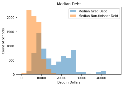
Debt for finishers is higher than it is for non-finishers because finishers tend to complete more credits and pay more tuition. For non-finishers, the distribution is unimodal and fairly compact, with the mode between $2,500 and $5,000. For graduates, debt is bimodal, one between $7,500 and $10,000 and another between $22,500 and $25,000 and a long tail, extending past $40,000. But how does it compare at different kinds of institutions?
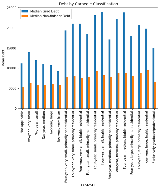
Graduates at four year institutions of all sizes generally have higher debt than those at two year institutions. Residential schools also have higher rates of median debt. The overall cost of a four year, residential program will be consistently higher than that of a two year, non-residential program. The average debt for non-finishers, however, is much more similar for all institution types, clustered just above $5000. One surprise: grad only institutions have lower median debt than most four year institutions, despite the fact that grad school is often expensive and paid for with loans.
2. Are there regional trends in graduation rates?
Schools are divided into regions: U.S. Service Schools, New England, Mid East, Great Lakes, Plains, Southeast, Southwest, Rocky Mountains, Far West, and Outlying Areas. Each region likely differs in the kinds of students that attend, so there may be differences in the graduation rates for each region.
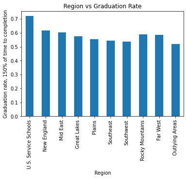
The most notable trend is that the service academies have much higher rates of graduation than any other region; this is likely due to their relatively small number and high selectivity. New England has the highest average graduation rate, even though it has a disproportionate number of colleges, and outlying areas (including mostly schools in US territories) have the lowest.
3. Does the selectivity of an institution (e.g., acceptance rate and SAT scores) correlate with its graduation rates?
In general, more selective institutions should likely have higher graduation rates. Let’s investigate the extent to which this is true. First, we’ll look at SAT scores.
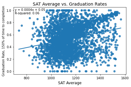
While there is a slight overall positive trend, differences in SAT averages explain only 6% of the variance in graduation rates. Let's look at the graduation rate just at four year institutions, where SAT scores are generally more frequently used.
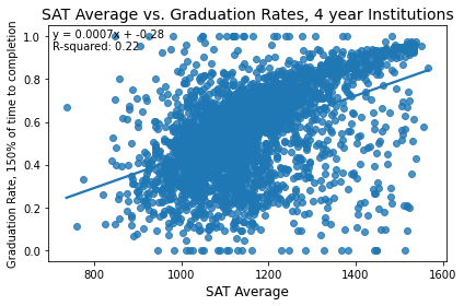
The strength of the relationship increases, but it is still not a strong relationship, although the general trend is that higher average SAT scores correspond to higher graduation rates.
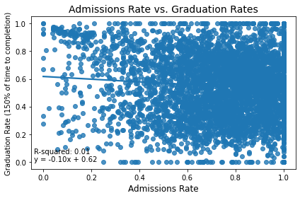
Admissions rate has less predictive power than SAT average does on graduation rate. Both of these findings are rather surprising! It makes sense that more selective schools would have higher graduation rates, because they select the top students from their applicant pools. The ETS also claims that the SAT is predictive of college success but that doesn't seem to be necessarily true.
4. Do public vs. private vs. for-profit institutions show distinct patterns in costs, debt, or graduation rates?
To answer this question simply: yes, they differ quite a bit. To come to this conclusion, I made a series of violin plots; violin plots are preferable to box plots, for example, because they show much more information about the shape of the distribution; the range and median are easy to identify, but one can also see the distribution of modal values and see how the distribution is spread out or compacted.
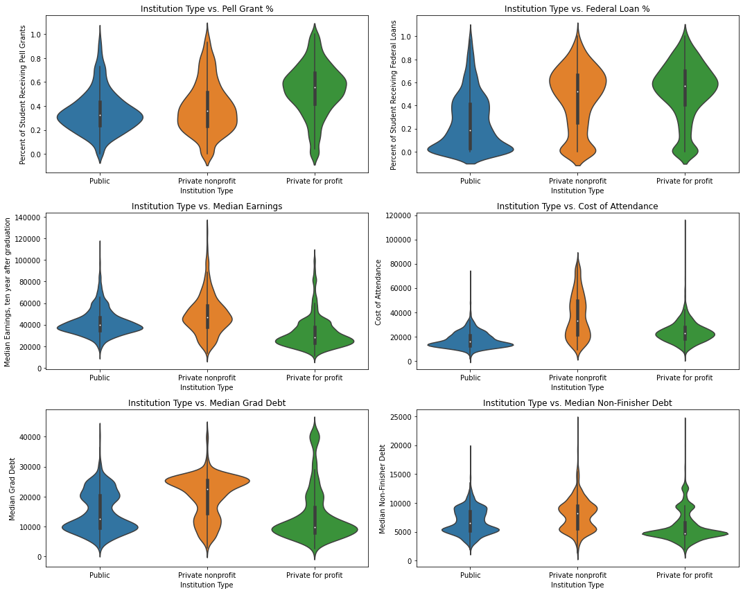
Pell grants are more common at private for profit institutions, as are federal loans; private nonprofits also have substantial number of students using private loans, although students at public schools are less likely to use either federal loans or Pell grants.
Public and nonprofit private institutions have similar distributions of median incomes after ten years, while for profit private institutions have lower median future wages. There are private institutions at almost every price point, but public ones are generally the least expensive.
Students at private nonprofit institutions generally have a higher debt burden than those at the other two types. Median debt for non-finishers is more similar across all three institution types, with two concentrations around $5000 and $10000.
5. What factors drive graduation rates?
To answer this question, I built a random forest model, described in the next two sections.
Section 3: Methodology
Data Preprocessing:
To conduct the analysis, I first needed to wrangle the data into a usable format. To do so, I imported the needed libraries, read in the data, and defined some functions to clean the data. The cleaning functions do two major tasks: first, a number of attributes that are spread across multiple columns are combined into one column. For example, graduation rate, as measured by 150% of time to completion for the average degree program, comes divided into one column for 4 year institutions and one for less than four year institutions. While there are interesting differences between these metrics, for my purposes, I'm most interested in the overall rate of completion, so I combined them into one column. To do this, I used the ‘forward fill’ function on the relevant columns and created a new column for the combined graduation rate metric.
Second, I replaced a common kind of missing data, the 'PrivacySupressed' value, with NaN to make it easier to spot and work with. A school will have 'PrivacySupressed' as a value when there are too few students in a group such that reporting the value might compromise the anonymity of the students in question. This happens a lot for small schools or small subsets of student demographics. However, 'PrivacySupressed' as a value often complicates analysis, because it forces numeric columns to be strings. The issue of converting the column type will be dealt with later down the line.
There isn't a single school that has complete data for the 2021-2022 school year, so it was impossible to do a complete case analysis with just one year’s data. Instead, I supplemented the data with values pulled from previous years using the last observation carried forward (LOCF) method of imputation. To do so, I added a tag for the year and used the ‘combine first’ function . ‘Combine first’ preserves every data point in the first DataFrame first, then replaces any NaNs with data from the second DataFrame; when combining year, the most recent year is the first DataFrame and the previous year is the second one and the last observation will be carried forward. Doing this ensures that the most recent data is what's always retained first, while any missing values can be supplemented. I used data from 2017-2022 (five years’ worth) to provide as much complete data as possible while maintaining the integrity of the data.
Combining data across years comes with one possible complication for any data reported as a dollar value; inflation decreases the value of money from year to year, and college tuition infamously rises at a rate faster than inflation. Luckily, the data for median income after graduation, faculty pay, cost of tuition, and debt after finishing are all variables with fairly complete data in the first year of the dataset; at most, about 2,500 schools are missing one or more of these financial metrics, and it's much less for many metrics (the one with the most missing is faculty salaries, which are, unfortunately for the faculty, easily the most stable over time). Using one additional year of data alone reduces the amount of school missing data on, for example, debt after finishing from around 1,600 schools to about 600. While changes in the value of money happen, the effect of inflation isn't so large as to render the data useless, and filling in from previous years is the most reasonable approach to balance the need for additional data with the need for accuracy in data. I also limit the number of years used to fill in missing values to four additional years, again to strike a balance between missing data and accuracy in the data.
Another potential issue is that the values will fluctuate wildly from year to year. This is always possible and is especially significant for very small schools; if a school only has cohorts of ten students, the graduation rate may vary by 10% easily. However, there are relatively few schools of that size, and most metrics are likely stable across time to a degree that makes analysis possible, at least. Again, the trade off is between more complete data and perfectly accurate data; my approach allows a reasonable balance of both.
Ultimately, combining across years gives a much more complete picture of each relevant metric in the data than is captured by just one year's worth. The creators of the College Scoreboard dataset recognize this because they sometimes use pooled metrics across years (such as a two year pooled graduation rate) to smooth out minor fluctuations. Combining across years gives a more complete picture, without making major sacrifices to data quality. Using five years of data gave me complete data for over 5,000 schools on the relevant metrics.
Implementation:
To predict graduation rates, a Random Forest model was used because of its superior performance compared to linear regression and elastic net models in preliminary tests. This decision was based on the R-squared metric, which indicated that the Random Forest model explained a larger proportion of the variance in graduation rates than the other classes of models. The model was trained on a subset of the data and evaluated on a separate test set to assess its predictive accuracy.
Feature importance analysis was conducted to identify the most influential predictors of graduation rates. Two primary methods were employed:
Drop-Column Analysis: Each predictor was systematically removed from the model, and the resulting change in R-squared was measured. A larger decrease in R-squared indicated a more important predictor.
Built-in Feature Importance: The Random Forest model's inherent feature importance scores were utilized, providing a direct measure of how much each feature contributes to the model's decision-making process.
Refinement:
The model was constructed using the following hyperparameters, which were tuned using grid search with cross-validation to optimize performance:
n_estimators: The number of trees in the forest. Values tested: 100, 200, 300.
max_depth: The maximum depth of each tree. Values tested: None, 10, 20, 30.
min_samples_split: The minimum number of samples required to split an internal node. Values tested: 2, 5, 10.
min_samples_leaf: The minimum number of samples required to be at a leaf node. Values tested: 1, 2, 4.
After conducting a grid search to optimize hyperparameters, the Random Forest model achieved its best performance with the following configuration: maximum tree depth was unrestricted, the minimum number of samples required to be at a leaf node was 4, the minimum number of samples required to split an internal node was 2, and the number of trees in the forest was 300. This optimized model demonstrated a reasonable ability to predict graduation rates, yielding an R-squared value of 0.5232 on the test set. The mean squared error of 0.0253 indicates a moderate degree of error in the predictions.
Section 4: Results
Model Evaluation and Validation:
The Random Forest model, trained on a diverse set of predictors, demonstrated a moderate ability to predict graduation rates, achieving an R-squared of 0.5232 and a mean squared error (MSE) of 0.0253. While the R-squared value indicates that the model explains 52.32% of the variance in graduation rates, it's important to note that the MSE suggests a certain degree of error in the predictions.
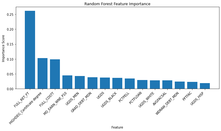
Feature Importance:
I wanted to know what variables are most important to my model, similar to the coefficient weights from a linear model. However, it is less straightforward for random forest regression. I need to systematically drop each predictor and compare the r-squared it returns; if dropping the variable lowers r-squared, the variable is an important predictor and if there's little change, it's less important as a predictor.
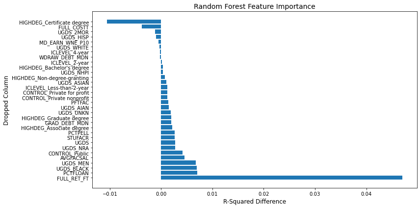
Retention rate is far and away the most significant factor; dropping it from the model worsens the model performance more than any other predictor. There is also a built-in measure of importance that measures the impact of shuffling the values for a particular predictor; if shuffling values changes the predictive power of the model, then the feature is important.
This version of feature importance also picks out retention rates as the most important predictor. Let's look more closely at the relationship using a partial dependence plot. This plot can identify the relationship between one predictor and the outcome when all other predictors are held constant.
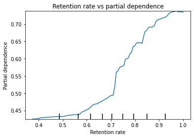
The Y axis of the partial dependence plot is the expected level of the outcome at a given level of the retention rate averaged across other factors. Higher retention is associated with higher graduation rate. The relationship looks like a series of small, nearly linear segments with different rates of change. Increases in retention rates between .7 and .8 lead to the fastest increases in graduation rate before leveling off.
In summary, feature importance analysis revealed several key drivers of graduation rates within the model.
Retention Rate: As expected, retention rate emerged as the most significant predictor, with a substantial drop in model performance observed when this feature was removed. This underscores the critical role of student persistence in achieving graduation.
Federal Loan Usage: The percentage of students receiving federal loans was another influential factor. This suggests that financial aid plays a vital role in supporting students through to graduation.
Institutional Control: The type of institutional control (public, private non-profit, or private for-profit) also exhibited a notable impact on graduation rates, indicating that the governance and financial structure of an institution can affect student outcomes.
Additional factors like faculty-to-student ratio, percentage of full-time faculty, and average faculty salary also showed some degree of importance, although their impact was less pronounced than retention rate, Pell Grant usage, and institutional control.
Justification of Results:
The selection of the Random Forest model was justified by its superior performance compared to linear regression and elastic net models in preliminary testing. The R-squared values for the Random Forest model were consistently higher, indicating that it more closely approximated the relationships between predictors and graduation rates, possibly due to the presence of interactions or non-linear relationships which were not included in these other classes of models.
Section 5: Conclusion
Reflection:
I was able to answer several questions about how schools compare across the College Scorecard that may be able to help a high school junior or senior decide on the best college for them. Location does matter, but I would argue that retention rate is a better predictor of graduation outcomes than selectivity is; retention rate came out as the clearest factor in the random forest model, while the linear relationships between SAT average and admissions rates were not particularly strong.
Private non-profit schools have higher median earnings (and higher values for other earnings quantiles), but that corresponds to a higher cost of tuition and higher debt after leaving the school. Public and private for-profit institutions have somewhat lower median earnings ten years after graduation, but that is counterbalanced by generally lower tuition costs and thus lower loan balances at the end of school. How one decides to choose between each institution type depends on what one weighs as more important: higher earning potential with higher debt, or lower debt and (somewhat) lower earning potential.
Additionally, the type of school (residential vs nonresidential) also impacts debt after leaving school. Shorter, non-residential program graduates have lower debt loads. Again, what a high school senior does with this information depends on what they value: someone who values the residential experience highly may still want to attend such an institution, even though the average grad has more debt.
The analysis revealed that retention rate stands as the most important predictor of graduation success, underscoring the importance of fostering supportive environments where students are encouraged to persist in their academic pursuits. Furthermore, the significant impact of Pell Grant usage highlights the importance of financial aid on improving graduation outcomes for economically disadvantaged students. The differing patterns observed across public, private non-profit, and private for-profit institutions emphasize the diverse nature of the higher education landscape, highlighting the need for tailored approaches to support students in different settings.
Improvement:
While this analysis has provided valuable insights, there are opportunities for further exploration and refinement. A deeper investigation into the complex relationship between institution type (public, private non-profit, for-profit) and earnings outcomes could offer a more nuanced understanding of the long-term financial benefits associated with different educational paths. Additionally, analyzing potential interaction effects between predictors (e.g., how the impact of Pell grants varies across different institution types) could reveal hidden complexities within the data.
Incorporating data from multiple years would enable a longitudinal analysis, shedding light on trends over time and revealing how institutional factors and student outcomes might be evolving. Furthermore, expanding the analysis to include additional variables, such as student academic preparation or pre-college socioeconomic status, could enhance our understanding of the factors contributing to student success.